Explore Genotype-Phenotype Associations

Pantograph offers interactive ways in linking genetic to phenotypic variation, on single variants as well as on long haplotypes.

Stratified metadata distributions

Pantograph offers to plot trait value distributions stratified by genetic data: by presence/absence variation between the graph paths, or by variant alleles between the samples from variant tracks.

Variation between graph paths

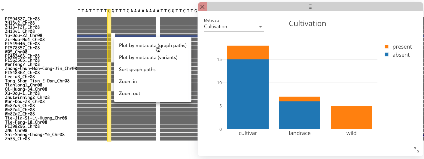
By right-clicking on a column, select "Plot by metadata (graph paths)" and Pantograph groups the paths by presence/absence of sequence in the selected column. For each group, a stacked bar plot for categorical or a boxplot for numerical data is plotted in an extra window for any metadata that you can choose from the dropdown in the top left corner.

Variation between genotyped samples

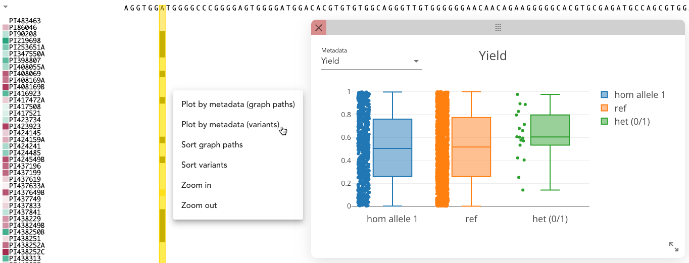
By right-clicking on a column that includes variants in the variant tracks, select "Plot by metadata (variants)" and Pantograph groups the variant track samples by their alleles for the selected variant. For each group, a bar plot for categorical or a boxplot for numerical data is plotted in an extra window for any metadata that you can choose from the dropdown in the top left corner.

Clustering pangenome regions

Pantograph allows users to associate long stretches of sequence (haplotypes) with phenotypic variation through the following steps:

1. Select a region (details below): Define a custom region in the pangenome.
2. Assess sequence lengths: Review sequence lengths for each track and assign a pipeline name for easy identification on the very top.
3. Run clustering: A bioinformatics pipeline generates a phylogenetic tree in the background.
4. Track progress: Monitor the pipeline's status on the Pipeline page.
5. View results: Once completed, the phylogenetic tree is accessible on the Pipeline page under the pipeline's name. It can be downloaded in newick format, or interactively viewed in the Tree Window.
6. Explore the clustering: The phylogenetic tree can be interactively explored in the Tree Window. Tracks are automatically sorted based on the order of samples in the clustering, from the top leaf to the bottom leaf. This sorting order is also represented as an added metadata category.
7. Subtrees can be selected and the phenotypic distributions of samples between the subtrees can be plotted and compared to each other.

Select a region

To select a region, hold the Shift key, then click and drag the mouse while keeping the button pressed. The selected region will be highlighted with a yellow box, and a menu will appear offering the option to perform clustering.

INFO

The clustering process includes all currently visible tracks, such as graph paths and/or variant tracks. For variant tracks, a pseudo-sequence is generated by integrating the respective variations directly into the reference sequence.

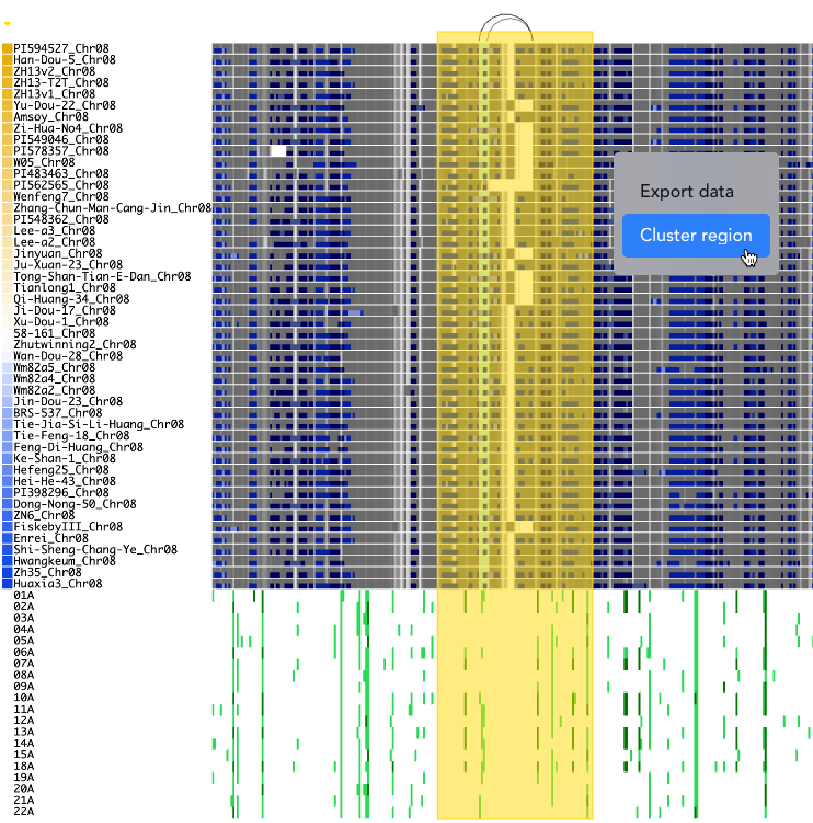
In the next step, the start and end positions of the selected graph paths, as well as those of the reference genome for the variant tracks, are extracted. The resulting sequence lengths are displayed in a table, allowing users to check for consistency.

INFO

Tracks are not included in the clustering if there are:

• non-unique positions: Start or end positions that are not unique due to duplications are excluded from the analysis, and the corresponding tracks will not be included in the clustering. This ensures that ambiguous combinations and multiple sequences per graph path are avoided.
• unknown positions: Tracks with large stretches of absent sequence may have unknown start or end positions. These tracks will also be excluded from clustering.

Moreover, the samples included in summarized tracks, even if the track is activated, are not included in the clustering.

TIP

To include most visible tracks in the clustering, select start and end positions that are outside duplicated regions and ensure that most tracks have coverage in the chosen region, especially the reference paths from the variant tracks. If the reference path does not have unique start/end coordinates, variant tracks relative to that reference will not be part of the clustering.

Tree Window

The Tree Window allows for the interactive exploration of phylogenetic trees.

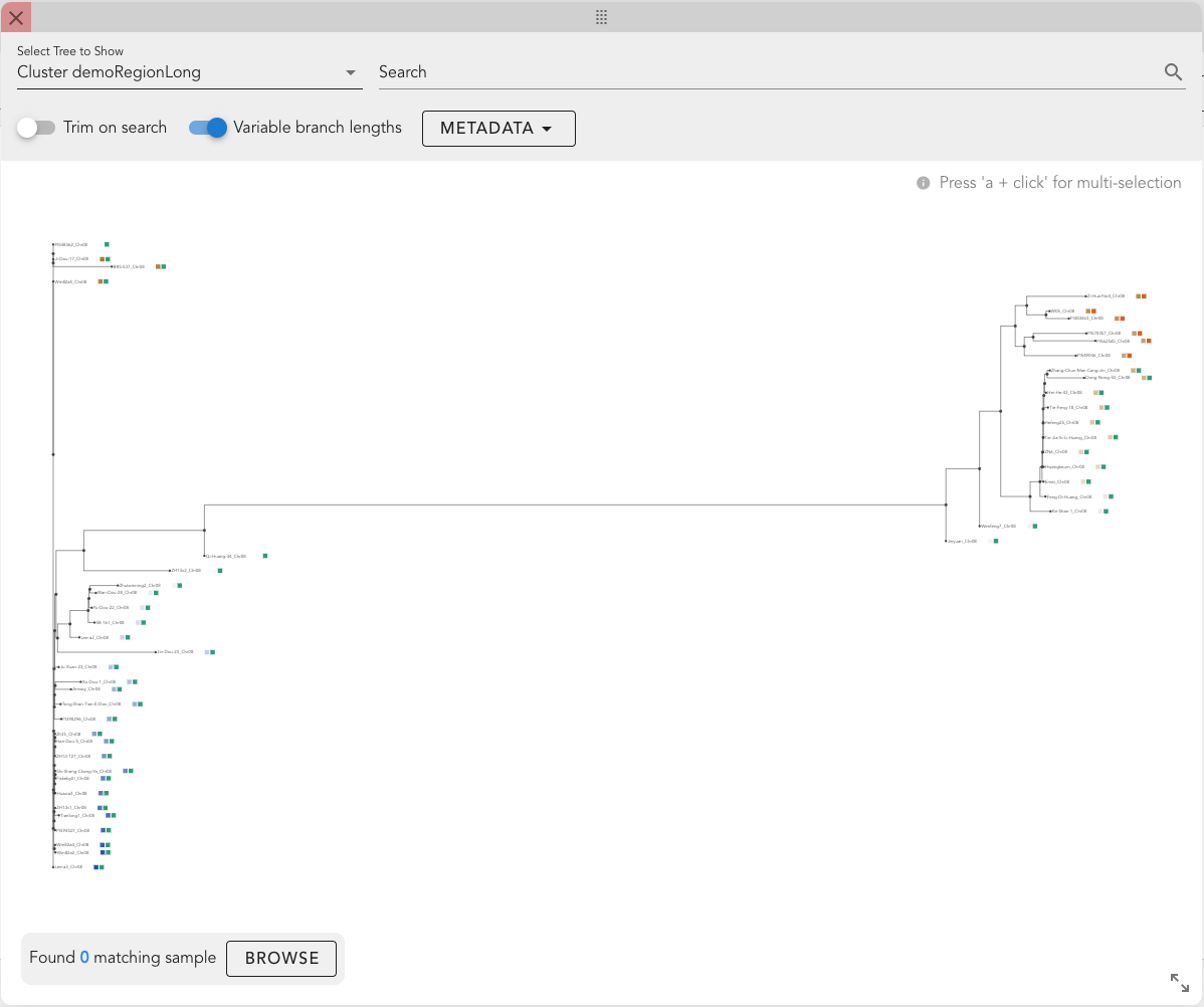
Features

• Tree Selection: Choose a tree to display. Available options typically include a chromosome-wide tree ("Chr-wide tree"), trees generated from clustering pipelines, or custom trees (contact Computomics to upload your own).
• Search Bar: Enter a comma-separated list of track names (partial matches allowed) to highlight matching samples.
• Trim on Search: Restrict the view to only the subtree containing samples that match the search criteria.
• Variable Branch Lengths: Toggle between variable and fixed branch lengths.
• Metadata Display: Select metadata categories to display as heat maps next to track names (i.e., leaf labels).
• Tree Canvas: The main display area for visualizing the tree.
• Browse Button: Indicates the number of tracks available in the currently selected subtree (or the entire tree if no selection is made). Clicking "Browse" closes the Tree Window and displays only the selected tracks in the Graph View.

TIP

If the tree is dragged outside the visible area, you can reposition it by selecting "Center Tree" from the right-click menu.

INFO

Bootstrap values
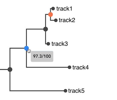
Bootstrap values, if specified in the Newick file, are displayed when hovering over internal nodes. Nodes with bootstrap values below 90% are highlighted in red, indicating areas of higher uncertainty in the tree topology.

Selecting subtrees and compare phenotypic distributions

Users can define groups of samples by selecting and combining subtrees, then visualize their phenotypic distributions.

Selecting Subtrees

Single Subtree Selection: Left-click on an internal node to select all leaf nodes within the corresponding subtree.

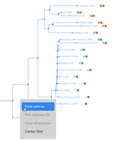
Combining Subtrees: To add another subtree to the selection, hold the 'A' key while clicking on an additional internal node.

Finalizing Selection: Once a group of samples is selected, right-click and choose "New Subtree" from the menu. You can assign a label to this group.

Additional groups can be created using the same process.

Plotting Phenotypic Distributions

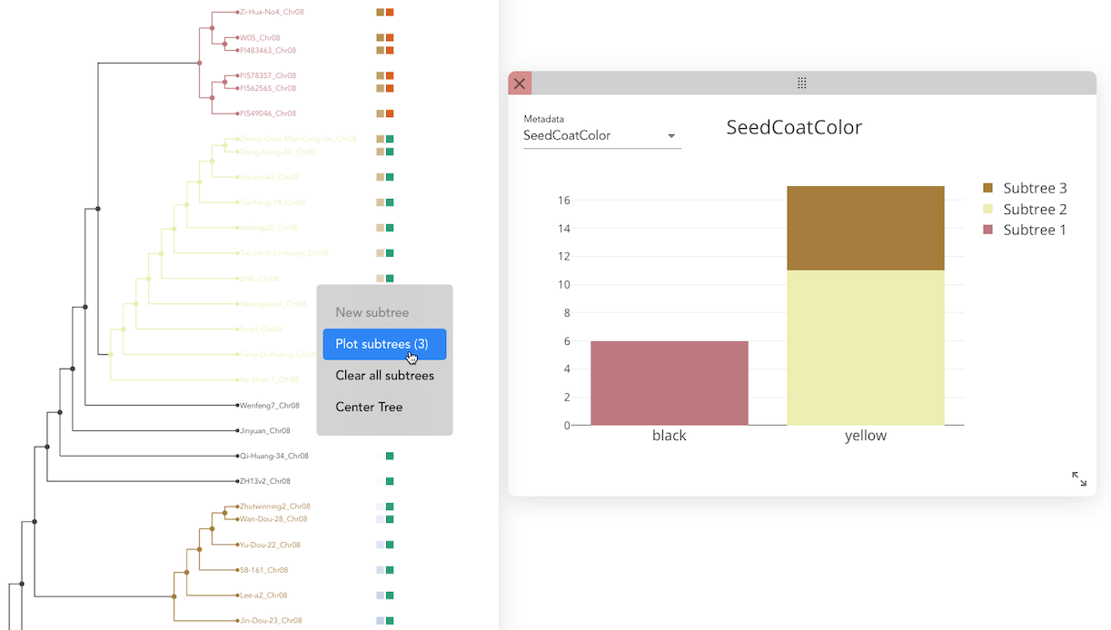
1. After defining all groups, click "Plot Subtree" to open the plot window.
2. Select a metadata category to visualize.
3. The phenotypic distributions for the sample groups are displayed as:

• A stacked bar plot for categorical data.
• A box plot for quantitative data.

This allows for an intuitive comparison of phenotypic traits across different sample groups.